Deproject
Deproject is a CIAO Sherpa extension package to facilitate
deprojection of two-dimensional annular X-ray spectra to recover the
three-dimensional source properties. For typical thermal models this would
include the radial temperature and density profiles. This basic method
has been used extensively for X-ray cluster analysis and is the basis for the
XSPEC model projct. The deproject module brings this
functionality to Sherpa as a Python module that is straightforward to use and
understand.
The deproject module uses specstack to allow for manipulation of
a stack of related input datasets and their models. Most of the functions
resemble ordinary Sherpa commands (e.g. set_par, set_source, ignore)
but operate on a stack of spectra.
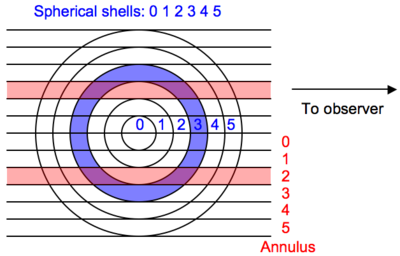
The basic physical assumption of deproject is that the extended source
emissivity is constant and optically thin within spherical shells whose radii
correspond to the annuli used to extract the specta. Given this assumption one
constructs a model for each annular spectrum that is a linear volume-weighted
combination of shell models. The geometry is illustrated in the figure below
(which would be rotated about the line to the observer in three-dimensions):
Model creation
It is assumed that prior to starting deproject the user has extracted
source and background spectra for each annulus. By convention the annulus
numbering starts from the inner radius at 0 and corresponds to the dataset
id used within Sherpa. It is not required that the annuli include the
center but they must be contiguous between the inner and outer radii.
Given a spectral model M[s] for each shell s, the source model for
dataset a (i.e. annulus a) is given by the sum over s >= a of
vol_norm[s,a] * M[s] (normalized volume * shell model). The image above
shows shell 3 in blue and annulus 2 in red. The intersection of (purple) has a
physical volume defined as vol_norm[3,2] * v_sphere where v_sphere is the
volume of the sphere enclosing the outer shell.
The bookkeeping required to create all the source models is handled by the
deproject module.
Fitting
Once the composite source models for each dataset are created the fit analysis can begin. Since the parameter space is typically large the usual procedure is to initally fit using the “onion-peeling” method:
- First fit the outside shell model using the outer annulus spectrum
- Freeze the model parameters for the outside shell
- Fit the next inward annulus / shell and freeze those parameters
- Repeat until all datasets have been fit and all shell parameters determined.
From this point the user may choose to do a simultanenous fit of the shell
models, possibly freezing some parameters as needed. This process is made
manageable with the specstack methods that apply normal Sherpa
commands like freeze or set_par to a stack of spectral datasets.
Densities
Physical densities (cm^-3) for each shell can be calculated with
deproject assuming the source model is based on a thermal model with the
“standard” normalization (from the XSPEC documentation):
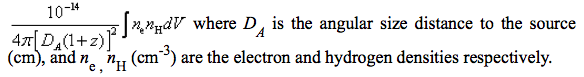
Inverting this equation and assuming a constant ratio of N_H to electrons:
n_e = sqrt(norm * 4*pi * DA^2 * 1e14 * (1+z)^2 / (volume * ne_nh_ratio))

norm        = model normalization from Sherpa fit
DA          = angular size distance (cm)
volume      = volume (cm^3)
ne_nh_ratio = 1.18
Recall that the model components for each volume element (intersection of the
annular cylinder a with the spherical shell s) are multiplied by a volume
normalization:
vol_norm[s,a] = v[s,a] / v_sphere
v_sphere = volume of sphere enclosing outer annulus
With this convention the volume used above in calculating the electron
density for each shell is always v_sphere.
Download
The deproject package is available for download at deproject.tar.gz. The M87 data needed to run the example
analysis is available as m87.tar.gz
The source is available on github at https://github.com/taldcroft/deproject.
Installation
The deproject package includes three Python modules that must be made
available to the CIAO python so that Sherpa can import them. The first step
is to untar the package tarball, change into the source directory, and initialize
the CIAO environment:
tar zxvf deproject-<version>.tar.gz
tar zxvf m87.tar.gz -C deproject-<version>/examples   # Needed for example / test script
cd deproject-<version>
source /PATH/TO/ciao/bin/ciao.csh
There are three methods for installing. Choose ONE of the three.
Simple:
The very simplest installation strategy is to just leave the module files in
the source directory and set the PYTHONPATH environment variable to point
to the source directory:
setenv PYTHONPATH $PWD
This method is fine in the short term but you always have to make sure
PYTHONPATH is set appropriately (perhaps in your ~/.cshrc file). And if you
start doing much with Python you will have PYTHONPATH conflicts and things
will get messy.
Better:
If you cannot write into the CIAO python library then do the following. These
commands create a python library in your home directory and install the
deproject modules there. You could of course choose another directory
instead of $HOME as the root of your python library.
mkdir -p $HOME/lib/python
python setup.py install --home=$HOME
setenv PYTHONPATH $HOME/lib/python
Although you still have to set PYTHONPATH this method allows you to install
other Python packages to the same library path. In this way you can make a
local repository of packages that will run within Sherpa.
Best:
If you have write access to the CIAO installation you can just use the CIAO python to install the modules into the CIAO python library. Assuming you are in the CIAO environment do:
python setup.py install
This puts the new modules straight in to the CIAO python library so that any time
you enter the CIAO environment they will be available. You do NOT need to set
PYTHONPATH.
Test
To test the installation change to the source distribution directory and do the following:
cd examples
sherpa
execfile('fit_m87.py')
plot_fit(0)
log_scale()
This should run through in a reasonable time and produce output indicating the onion-peeling fit. The plot should show a good fit.
Example: M87
Now we step through in detail the fit_m87.py script in the examples
directory to explain each step and illustrate how to use the deproject
module. This script should serve as the template for doing your own analysis.
This example uses extracted spectra, response products, and analysis results for the Chandra observation of M87 (obsid 2707). These were kindly provided by Paul Nulsen. Results based on this observation can be found in Forman et al 2005 and via the CXC Archive Obsid 2707 Publications list.
The first step is to tell Sherpa about the Deproject class and set a couple of constants:
from deproject import Deproject

redshift = 0.004233                     # M87 redshift
arcsec_per_pixel = 0.492                # ACIS plate scale
angdist = 4.9e25                        # M87 distance (cm) (16 Mpc)
Next we create a numpy array of the the annular radii in arcsec. The numpy.arange method here returns an array from 30 to 640 in steps of 30. These values were in pixels in the original spectral extraction so we convert to arcsec. (Note the convenient vector multiplication that is possible with numpy.)
radii = numpy.arange(30., 640., 30) * arcsec_per_pixel
The radii parameter must be a list of values that starts with the inner
radius of the inner annulus and includes each radius up through the outer
radius of the outer annulus. Thus the radii list will be one element
longer than the number of annuli.
Now the key step of creating the Deproject object dep. This
object is the interface to the all the deproject
methods used for the deprojection analysis.
dep = Deproject(radii, theta=75, angdist=angdist)
If you are not familiar with object oriented programming, the dep object is
just a thingy that stores all the information about the deprojection analysis
(e.g. the source redshift, PHA file information and the source model
definitions) as object attributes. It also has object methods
(i.e. functions) you can call such as dep.get_par(parname) or
dep.load_pha(file). The full list of attributes and methods are in the
deproject module documentation.
In this particular analysis the spectra were extracted from a 75 degree sector
of the annuli, hence theta=75 in the object initialization. For the
default case of full 360 degree annuli this is not needed. Because the
redshift is not a good distance estimator for M87 we also explicitly set the
angular size distance.
Now load the PHA spectral files for each annulus using the Python range
function to loop over a sequence ranging from 0 to the last annulus. The
load_pha() call is the first example of a deproject method
(i.e. function) that mimics a Sherpa function with the same name. In this
case dep.load_pha(file, annulus) loads the PHA file using the Sherpa load_pha
function but also registers the dataset in the spectral stack:
for annulus in range(len(radii)-1):
    dep.load_pha('m87/r%dgrspec.pha' % (annulus+1), annulus)
The annulus parameter is required in dep.load_pha() to support analysis
of multi-obsid datasets.
With the data loaded we set the source model for each of the spherical shells
with the set_source() method. This is one of the more complex bits of
deproject. It automatically generates all the model components for each
shell and then assigns volume-weighted linear combinations of those components
as the source model for each of the annulus spectral datasets:
dep.set_source('xswabs * xsmekal')
The model expression can be any valid Sherpa model expression with the following caveats:
- Only the generic model type should be specified in the expression. In typical Sherpa usage one generates the model component name in the model expression, e.g.
set_source("xswabs.abs1 * xsmekal.mek1"). This would create model components namedabs1andmek1. Indep.set_source()the model component names are auto-generated as<model_type>_<shell>.- Only one of each model type can be used in the model expression. A source model expression like “xsmekal + gauss1d + gauss1d” would result in an error due to the model component auto-naming.
Now the energy range used in the fitting is restricted using the stack version of the Sherpa ignore command. The notice command is also available.
dep.ignore(None, 0.5)
dep.ignore(1.8, 2.2)
dep.ignore(7, None)
Next any required parameter values are set and their freeze or thaw status are set.
dep.set_par('xswabs.nh', 0.0255)
dep.freeze("xswabs.nh")

dep.set_par('xsmekal.abundanc', 0.5)
dep.thaw('xsmekal.abundanc')

dep.set_par('xsmekal.redshift', redshift)
As a convenience if any of the model components have a
redshift parameter that value will be used as the default redshift for
calculating the angular size distance.
At this point the model is completely set up and we are ready to do the initial
“onion-peeling” fit. As for normal high-signal fitting with binned spectra we
issue the commands to set the optimization method, set the fit statistic, and
configure Sherpa to subtract the background when doing model fitting.
Finally the deproject fit() method is called to perform the fit.
set_method("levmar")                    # Levenberg-Marquardt optimization method
set_stat("chi2gehrels")                 # Gehrels Chi^2 fit statistic
dep.subtract()
dep.fit()
After the fit process each shell model has an association normalization that
can be used to calculate the densities. This is where the source angular
diameter distance is used. If the angular diameter distance is not set
explicitly in the original dep = Deproject(...) command then it is
calculated automatically from the redshift found as a source model
parameter. One can examine the values being used as follows:
print "z=%.5f angdist=%.2e cm" % (dep.redshift, dep.angdist)
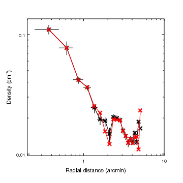
The electron density is then calculated with the get_density() method and
plotted in Sherpa:
density_ne = dep.get_density()
rad_arcmin = (dep.radii[:-1] + dep.radii[1:]) / 2.0 / 60.
add_curve(rad_arcmin, density_ne)
set_curve(['symbol.color', 'red', 'line.color', 'red'])
set_plot_xlabel('Radial distance (arcmin)')
set_plot_ylabel('Density (cm^{-3})')
limits(X_AXIS, 0.2, 10)
log_scale()
print_window('m87_density', ['format', 'png'])
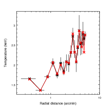
The temperature profile from the deproject can be plotted as follows:
kt = dep.get_par('xsmekal.kt')   # returns array of kT values
add_window()
add_curve(rad_arcmin, kt)
set_plot_xlabel('Radial distance (arcmin)')
set_plot_ylabel('Density (cm^{-3})')
The unphysical temperature oscillations seen here highlights a known issue with this analysis method.
In the images below the deproject results (red) are compared with values
(black) from an independent onion-peeling analysis by P. Nulsen using a custom
perl script to generate XSPEC model definition and fit commands. These
plots were created with the plot_m87.py script in the examples
directory. The agreement is good:
Example: Multi-obsid
A second example illustrates the use of deproject for a multi-obsid
observation of 3c186. It also shows how to set a background model for fitting
with the cstat statistic. The extracted spectral data for this example are
not yet publicly available.
The script starts with some setup:
import deproject

radii = ('2.5', '6', '17')
dep = deproject.Deproject(radii=[float(x) for x in radii])

set_method("levmar")
set_stat("cstat")
Now we read in the data as before with dep.load_pha(). The only difference
here is an additional loop over the obsids. The dep.load_pha() function
automatically extracts the obsid from the file header. This is used later in
the case of setting a background model.
obsids = (9407, 9774, 9775, 9408)
for ann in range(len(radii)-1):
    for obsid in obsids:
        dep.load_pha('3c186/%d/ellipse%s-%s.pi' % (obsid, radii[ann], radii[ann+1]), annulus=ann)
Create and configure the source model expression as usual:
dep.set_source('xsphabs*xsapec')
dep.ignore(None, 0.5)
dep.ignore(7, None)
dep.freeze("xsphabs.nh")

dep.set_par('xsapec.redshift', 1.06)
dep.set_par('xsphabs.nh', 0.0564)
Set the background model:
execfile("acis-s-bkg.py")
acis_s_bkg = get_bkg_source()
dep.set_bkg_model(acis_s_bkg)
Fit the projection model:
dep.fit()
To Do
- Use the Python logging module to produce output and allow for a verbosity setting. [Easy]
- Create and use more generalized
ModelStackandDataStackclasses to allow for general mixing models. [Hard]