M87¶

Now we step through in detail the fit_m87.py script in the examples directory to explain each step and illustrate how to use the deproject module. This script should serve as the template for doing your own analysis.

This example uses extracted spectra, response products, and analysis results for the Chandra observation of M87 (obsid 2707). These were kindly provided by Paul Nulsen. Results based on this observation can be found in Forman et al 2005 and via the CXC Archive Obsid 2707 Publications list.

The examples assume this is being run directly from the Sherpa shell, which has already imported the Sherpa module. If you are using IPython or a Jupyter notebook then the following command is needed:

>>> from sherpa.astro.ui import *

Set up¶

The first step is to load in the Deproject class:

>>> from deproject import Deproject

and then set a couple of constants (note that both the angular-diameter distance and thta values must be Astropy quantites):

>>> from astropy import units as u
>>> redshift = 0.004233                     # M87 redshift
>>> angdist = 16 * u.Mpc                    # M87 distance
>>> theta = 75 * u.deg                      # Covering angle of sectors

Next we create an array of the the annular radii in arcsec. The numpy.arange method here returns an array from 30 to 640 in steps of 30. These values were in pixels in the original spectral extraction so we multiply by the pixel size (0.492 arcseconds) to convert to an angle.:

>>> radii = numpy.arange(30., 640., 30) * 0.492 * u.arcesc

The radii parameter must be a list of values that starts with the inner radius of the inner annulus and includes each radius up through the outer radius of the outer annulus. Thus the radii list will be one element longer than the number of annuli.

>>> print(radii)
[ 14.76  29.52  44.28  59.04  73.8   88.56 103.32 118.08 132.84 147.6
 162.36 177.12 191.88 206.64 221.4  236.16 250.92 265.68 280.44 295.2
 309.96] arcsec

Now the key step of creating the Deproject object dep. This object is the interface to the all the deproject methods used for the deprojection analysis.

>>> dep = Deproject(radii, theta=theta, angdist=angdist)

If you are not familiar with object oriented programming, the dep object is just a thingy that stores all the information about the deprojection analysis (e.g. the source redshift, PHA file information and the source model definitions) as object attributes. It also has object methods (i.e. functions) you can call such as dep.get_par(parname) or dep.load_pha(file). The full list of attributes and methods are in the deproject module documentation.

In this particular analysis the spectra were extracted from a 75 degree sector of the annuli, hence theta is set in the object initialization, where the units are set explicitly using the Astropy support for units. Note that this parameter only needs to be set if any of the annuli are sectors rather than the full circle. Since the redshift is not a good distance estimator for M87 we also explicitly set the angular size distance using the angdist parameter.

Load the data¶

Now load the PHA spectral files for each annulus using the Python range function to loop over a sequence ranging from 0 to the last annulus. The load_pha() call is the first example of a deproject method (i.e. function) that mimics a Sherpa function with the same name. In this case dep.load_pha(file, annulus) loads the PHA file using the Sherpa load_pha function but also registers the dataset in the spectral stack:

>>> for annulus in range(len(radii) - 1):
...    dep.load_pha('m87/r%dgrspec.pha' % (annulus + 1), annulus)

Note

The annulus parameter is required in dep.load_pha() to allow multiple data sets per annulus, such as repeated Chandra observations or different XMM instruments.

Create the model¶

With the data loaded we set the source model for each of the spherical shells with the set_source() method. This is one of the more complex bits of deproject. It automatically generates all the model components for each shell and then assigns volume-weighted linear combinations of those components as the source model for each of the annulus spectral datasets:

>>> dep.set_source('xswabs * xsmekal')

The model expression can be any valid Sherpa model expression with the following caveats:

Only the generic model type should be specified in the expression. In typical Sherpa usage one generates the model component name in the model expression, e.g. set_source('xswabs.abs1 * xsmekal.mek1'). This would create model components named abs1 and mek1. In dep.set_source() the model component names are auto-generated as <model_type>_<shell>.

Only one of each model type can be used in the model expression. A source model expression like "xsmekal + gauss1d + gauss1d" would result in an error due to the model component auto-naming.

Next any required parameter values are set and their freeze or thaw status are set.

>>> dep.set_par('xswabs.nh', 0.0255)
>>> dep.freeze('xswabs.nh')

>>> dep.set_par('xsmekal.abundanc', 0.5)
>>> dep.thaw('xsmekal.abundanc')

>>> dep.set_par('xsmekal.redshift', redshift)

As a convenience if any of the model components have a redshift parameter that value will be used as the default redshift for calculating the angular size distance.

Define the data to fit¶

Now the energy range used in the fitting is restricted using the stack version of the Sherpa ignore command. The notice command is also available.

>>> dep.ignore(None, 0.5)
>>> dep.ignore(1.8, 2.2)
>>> dep.ignore(7, None)

Define the optimiser and statistic¶

At this point the model is completely set up and we are ready to do the initial “onion-peeling” fit. As for normal high-signal fitting with binned spectra we issue the commands to set the optimization method and the fit statistic.

In this case we use the Levenberg-Marquardt optimization method with the \(\chi^2\) fit statistic, where the variance is estimated using a similar approach to XSPEC.

>>> set_method("levmar")
>>> set_stat("chi2xspecvar")
>>> dep.subtract()

Note

The chi2xspecvar statistic is used since the values will be compared to results from XSPEC.

Seeding the fit¶

We first try to “guess” a good starting point for the fit (since the default fit parameters, in particular the normalization, are often not close to the expected value). In this case the guess() method implements a scheme suggested in the projct documentation, which fits each annulus with an un-projected model and then corrects the normalizations for the shell/annulus overlaps:

>>> dep.guess()
Projected fit to annulus 19 dataset: 19
Dataset               = 19
...
Change in statistic   = 4.60321e+10
   xsmekal_19.kT   2.748        +/- 0.0551545
   xsmekal_19.Abundanc   0.429754     +/- 0.0350466
   xsmekal_19.norm   0.00147471   +/- 2.45887e-05
Projected fit to annulus 18 dataset: 18
Dataset               = 18
...
Change in statistic   = 4.61945e+10
   xsmekal_18.kT   2.68875      +/- 0.0543974
   xsmekal_18.Abundanc   0.424198     +/- 0.0335045
   xsmekal_18.norm   0.00147443   +/- 2.43454e-05
...
Projected fit to annulus 0 dataset: 0
Dataset               = 0
...
Change in statistic   = 2.15043e+10
   xsmekal_0.kT   1.57041      +/- 0.0121572
   xsmekal_0.Abundanc   1.05816      +/- 0.0373779
   xsmekal_0.norm   0.00152496   +/- 2.93297e-05

As shown in the screen output, the guess routine fits each annulus in turn, from outer to inner. After each fit, the normalization (the xsmekal_*.norm terms) are adjusted by the filling factor of the shell.

Note

The guess step is optional. Parameter values can also be set, either for an individual annulus with the Sherpa set_par function, such as:

set_par('xsmekal_0.kt', 1.5)

or to all annuli with the Deproject method set_par():

dep.set_par('xsmekal.abundanc', 0.3)

The data can be inspected using normal Sherpa commands. The following shows the results of the guess for dataset 0, which corresponds to the inner-most annulus (the datasets attribute can be used to map between annuus and dataset identifier).

>>> set_xlog()
>>> plot_fit(0)

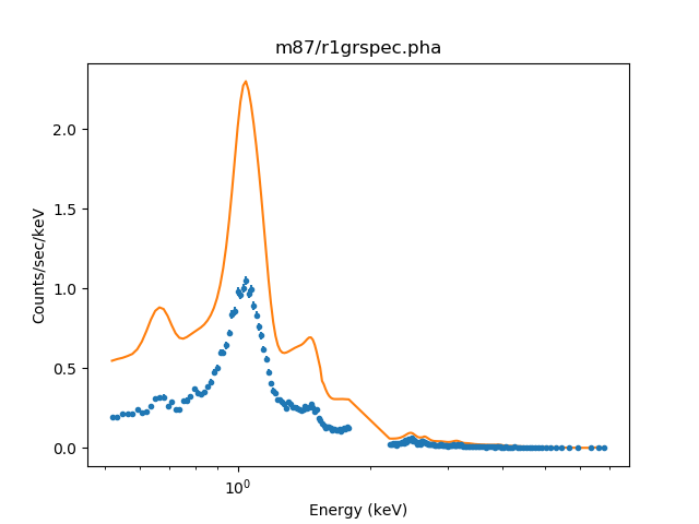
The overall shape of the model looks okay, but the normalization is not (since it has been adjusted by the volume-filling factor of the intersection of the annulus and shell). The gap in the data around 2 keV is because we explicitly excluded this range from the fit.

Note

The Deproject class also provides methods for plotting each annulus in a separate window, such as plot_data() and plot_fit().

Fitting the data¶

The fit() method performs the full onion-skin deprojection (the output is similar to the guess method, with the addition of parameters being frozen as each annulus is processed):

>>> onion = dep.fit()
Fitting annulus 19  dataset: 19
Dataset               = 19
...
Reduced statistic     = 1.07869
Change in statistic   = 1.29468e-08
   xsmekal_19.kT   2.748        +/- 0.0551534
   xsmekal_19.Abundanc   0.429758     +/- 0.0350507
   xsmekal_19.norm   0.249707     +/- 0.00416351
Freezing xswabs_19
Freezing xsmekal_19
Fitting annulus 18  dataset: 18
Dataset               = 18
...
Reduced statistic     = 1.00366
Change in statistic   = 13444.5
   xsmekal_18.kT   2.41033      +/- 0.274986
   xsmekal_18.Abundanc   0.375824     +/- 0.136926
   xsmekal_18.norm   0.0551815    +/- 0.00441495
Freezing xswabs_18
Freezing xsmekal_18
...
Freezing xswabs_1
Freezing xsmekal_1
Fitting annulus 0  dataset: 0
Dataset               = 0
...
Reduced statistic     = 2.72222
Change in statistic   = 12115.6
   xsmekal_0.kT   1.63329      +/- 0.0278325
   xsmekal_0.Abundanc   1.1217       +/- 0.094871
   xsmekal_0.norm   5.7067       +/- 0.262766
Change in statistic   = 13699.6
   xsmekal_0.kT   1.64884      +/- 0.0242336
   xsmekal_0.Abundanc   1.14629      +/- 0.0903398
   xsmekal_0.norm   5.68824      +/- 0.245884
...

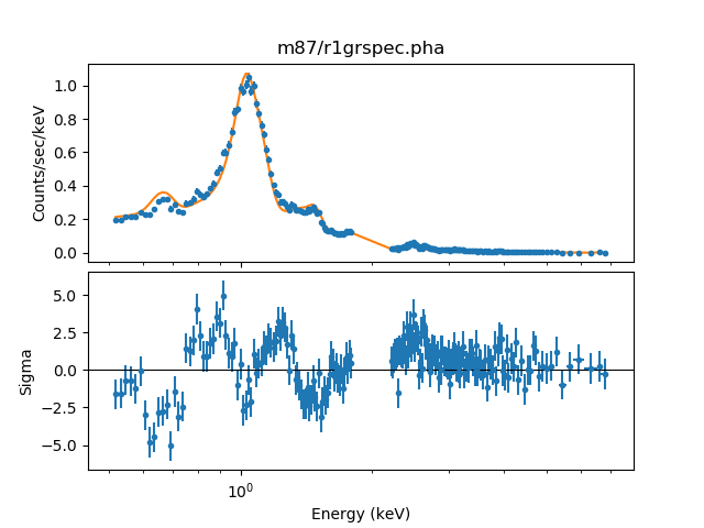
The fit to the central annulus (dataset 0) now looks like:

>>> plot_fit_delchi(0)

After the fit process each shell model has an association normalization that can be used to calculate the densities. This is where the source angular diameter distance is used. If the angular diameter distance is not set explicitly in the original dep = Deproject(...) command then it is calculated automatically from the source redshift and an assumed Cosmology, which if not set is taken to be the Planck15 model provided by the astropy.cosmology module.

One can examine the values being used as follows (note that the angdist attribute is an Astropy Quantity):

>>> print("z={:.5f} angdist={}".format(dep.redshift, dep.angdist))
z=0.00423 angdist=16.0 Mpc

New in version 0.2.0 is the behavior of the fit method, which now returns an Astropy table which tabulates the fit results as a function of annulus. This includes the electron density, which can also be retrieved with get_density(). The fit results can also be retrieved with the get_fit_results() method.

>>> print(onion)
annulus rlo_ang rhi_ang ...     xsmekal.norm          density
         arcsec  arcsec ...                           1 / cm3
------- ------- ------- ... ------------------- --------------------
      0   14.76   29.52 ...  5.6882389946381275   0.1100953546292787
      1   29.52   44.28 ...  2.8089409208987233  0.07736622021374819
      2   44.28   59.04 ...   0.814017947154132  0.04164827967805805
      3   59.04    73.8 ...  0.6184339453006981  0.03630168106524076
      4    73.8   88.56 ...  0.2985327157676323 0.025221797991301052
      5   88.56  103.32 ... 0.22395312678845017 0.021845331641349316
    ...     ...     ... ...                 ...                  ...
     13  206.64   221.4 ... 0.07212121560592619 0.012396857131392835
     14   221.4  236.16 ... 0.08384338967492334  0.01336640115325031
     15  236.16  250.92 ... 0.07104455447410102 0.012303975980575187
     16  250.92  265.68 ... 0.08720295254137615 0.013631563529090736
     17  265.68  280.44 ... 0.09192970392746878 0.013996131292837352
     18  280.44   295.2 ... 0.05518150227052414 0.010843683594144967
     19   295.2  309.96 ... 0.24970680803387219 0.023067220584935984
Length = 20 rows

Inspecting the results¶

The electron density can be retrieved directly from the fit results, with the get_density() method:

>>> print(dep.get_density())
[ 0.11009535  0.07736622  0.04164828  0.03630168  0.0252218   0.02184533
  0.01525456  0.01224972  0.01942528  0.01936785  0.01905983  0.01568478
  0.01405426  0.01239686  0.0133664   0.01230398  0.01363156  0.01399613
  0.01084368  0.02306722] 1 / cm3

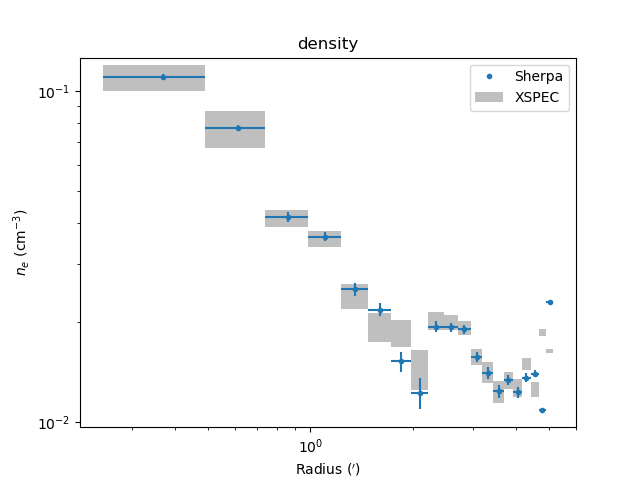
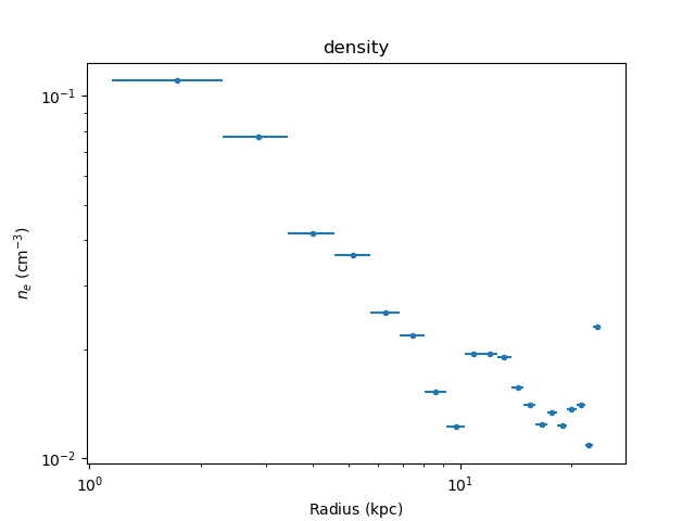
or plotted using density_plot():

>>> dep.density_plot()

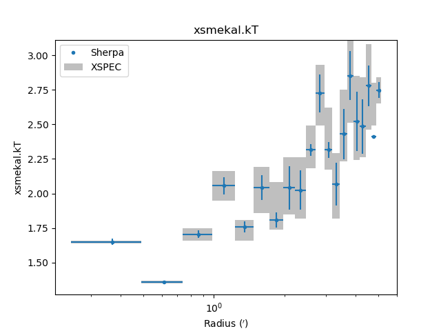
The temperature profile from the deprojection can be plotted using par_plot():

>>> dep.par_plot('xsmekal.kt')

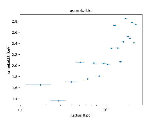
The unphysical temperature oscillations seen here highlights a known issue with this analysis method (e.g. Russell, Sanders, & Fabian 2008).

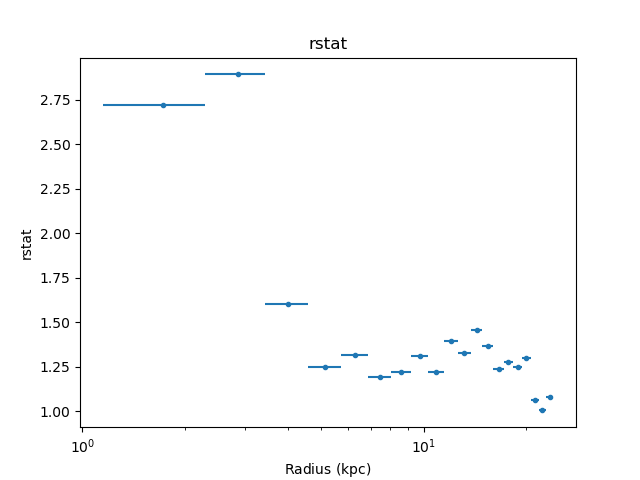
It can also be instructive to look at various results from the fit, such as the reduced statistic for each annulus (as will be shown below, there are fit_plot(), conf_plot(), and covar_plot() variants):

>>> dep.fit_plot('rstat')

Error analysis¶

Errors can also be calculated, on both the model parameters and the derived densities, with either the conf() or covar() methods. These apply the confidence and covariance error-estimation routines from Sherpa using the same onion-skin model used for the fit, and are new in version 0.2.0. In this example we use the covariance version, since it is generally faster, but confidence is the recommended routine as it is more robust (and calculates asymmetric errors):

>>> errs = dep.covar()

As with the fit method, both conf and covar return the results as an Astropy table. These can also be retrieved with the get_conf_results() or get_covar_results() methods. The columns depend on the command (i.e. fit or error results):

>>> print(errs)
annulus rlo_ang rhi_ang ...        density_lo             density_hi
         arcsec  arcsec ...         1 / cm3                1 / cm3
------- ------- ------- ... ----------------------- ----------------------
      0   14.76   29.52 ...  -0.0023299300992805777  0.0022816336635322065
      1   29.52   44.28 ...  -0.0015878693875514133  0.0015559288091097495
      2   44.28   59.04 ...  -0.0014852395638492444  0.0014340671599212054
      3   59.04    73.8 ...  -0.0011539611188859725    0.00111839214283211
      4    73.8   88.56 ...   -0.001166653616914693   0.001115024462355424
      5   88.56  103.32 ...  -0.0010421595234548324  0.0009946565126391325
    ...     ...     ... ...                     ...                    ...
     13  206.64   221.4 ...  -0.0005679816551559976  0.0005430748019680798
     14   221.4  236.16 ... -0.00048083556526315463 0.00046412880973027357
     15  236.16  250.92 ...  -0.0004951659664768401 0.00047599490797040934
     16  250.92  265.68 ...  -0.0004031089363366082  0.0003915259159180066
     17  265.68  280.44 ...  -0.0003647519140328147 0.00035548459401609986
     18  280.44   295.2 ...                     nan                    nan
     19   295.2  309.96 ... -0.00019648511719753958 0.00019482554589523096
Length = 20 rows

Note

With this set of data, the covariance method failed to calculate errors for the parameters of the last-but one shell, which is indicated by the presence of NaN values in the error columns.

The fit or error results can be plotted as a function of radius with the fit_plot(), conf_plot(), and covar_plot() methods (the latter two include error bars). For example, the following plot mixes these plots with Matplotlib commands to compare the temperature and abundance profiles:

>>> plt.subplot(2, 1, 1)
>>> dep.covar_plot('xsmekal.kt', clearwindow=False)
>>> plt.xlabel('')
>>> plt.subplot(2, 1, 2)
>>> dep.covar_plot('xsmekal.abundanc', clearwindow=False)
>>> plt.subplots_adjust(hspace=0.3)

../_images/m87_temperature_abundance.png

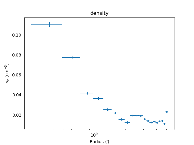
The derived density profile, along with errors, can also be displayed (the X axis is displayed using angular units rather than as a length):

>>> dep.covar_plot('density', units='arcmin')

Comparing results¶

In the images below the deproject results (blue) are compared with values (gray boxes) from an independent onion-peeling analysis by P. Nulsen using a custom perl script to generate XSPEC model definition and fit commands. These plots were created with the plot_m87.py script in the examples directory. The agreement is good (note that the version of XSPEC used for the two cases does not match):