Overview
The deproject module uses specstack to allow for manipulation of
a stack of related input datasets and their models. Most of the functions
resemble ordinary Sherpa commands (e.g. set_par, set_source, ignore)
but operate on a stack of spectra.
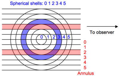
The basic physical assumption of deproject is that the extended source
emissivity is constant and optically thin within spherical shells whose radii
correspond to the annuli used to extract the specta. Given this assumption one
constructs a model for each annular spectrum that is a linear volume-weighted
combination of shell models. The geometry is illustrated in the figure below
(which would be rotated about the line to the observer in three-dimensions):
Model creation
It is assumed that prior to starting deproject the user has extracted
source and background spectra for each annulus. By convention the annulus
numbering starts from the inner radius at 0 and corresponds to the dataset
id used within Sherpa. It is not required that the annuli include the
center but they must be contiguous between the inner and outer radii.
Given a spectral model M[s] for each shell s, the source model for
dataset a (i.e. annulus a) is given by the sum over s >= a of
vol_norm[s,a] * M[s] (normalized volume * shell model). The image above
shows shell 3 in blue and annulus 2 in red. The intersection of (purple) has a
physical volume defined as vol_norm[3,2] * v_sphere where v_sphere
is the volume of the sphere enclosing the outer shell (as
discussed below).
The bookkeeping required to create all the source models is handled by the
deproject module.
Fitting
Once the composite source models for each dataset are created the fit analysis can begin. Since the parameter space is typically large the usual procedure is to initally fit using the “onion-peeling” method:
- First fit the outside shell model using the outer annulus spectrum
- Freeze the model parameters for the outside shell
- Fit the next inward annulus / shell and freeze those parameters
- Repeat until all datasets have been fit and all shell parameters determined.
From this point the user may choose to do a simultanenous fit of the shell
models, possibly freezing some parameters as needed. This process is made
manageable with the specstack methods that apply normal Sherpa
commands like freeze or set_par to a stack of spectral datasets.
Densities
Physical densities (\({\rm cm}^{-3}\)) for each shell can be calculated with
deproject assuming the source model is based on a thermal model with the
“standard” normalization (from the XSPEC documentation):
where \(D_A\) is the angular size distance to the source (in cm), \(z\) is the source redshift, and \(n_e\) and \(n_H\) are the electron and Hydrogen densities (in \({\rm cm}^{-3}\)).
Inverting this equation and assuming constant values for \(n_e\) and \(n_H\) gives
where \(V\) is the volume, \(n_H = \alpha n_e\), and \(\alpha\) is taken to be 1.18 (and this ratio is constant within the source).
Recall that the model components for each volume element (intersection of the
annular cylinder a with the spherical shell s) are multiplied by a
volume normalization:
where \(V_{\rm sphere}\) is the volumne of the sphere enclosing the outermost annulus.
With this convention the volume (\(V\)) used above in calculating the electron density for each shell is always \(V_{\rm sphere}\).