Combining shells

We now look at tie-ing parameters from different annuli (that is, forcing the temperature or abundance of one shell to be the same as a neighbouring shell), which is a technique used to try and reduce the “ringing” that can be seen in deprojected data (e.g. Russell, Sanders, & Fabian 2008 and seen in the temperature profile of the M87 data). Sherpa supports complicated links between model parameters with the link and unlink functions, and the Deproject class provides helper methods - tie_par() and untie_par() - that allows you to easily tie together annuli.

Starting from where the M87 example left off, we have:

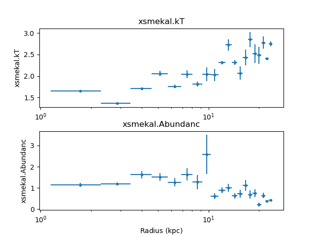
The get_shells() method lists the current set of annuli, and show that there are currently no grouped (or tied-together) annuli:

>>> dep.get_shells()
[{'annuli': [19], 'dataids': [19]},
 {'annuli': [18], 'dataids': [18]},
 {'annuli': [17], 'dataids': [17]},
 {'annuli': [16], 'dataids': [16]},
 {'annuli': [15], 'dataids': [15]},
 {'annuli': [14], 'dataids': [14]},
 {'annuli': [13], 'dataids': [13]},
 {'annuli': [12], 'dataids': [12]},
 {'annuli': [11], 'dataids': [11]},
 {'annuli': [10], 'dataids': [10]},
 {'annuli': [9], 'dataids': [9]},
 {'annuli': [8], 'dataids': [8]},
 {'annuli': [7], 'dataids': [7]},
 {'annuli': [6], 'dataids': [6]},
 {'annuli': [5], 'dataids': [5]},
 {'annuli': [4], 'dataids': [4]},
 {'annuli': [3], 'dataids': [3]},
 {'annuli': [2], 'dataids': [2]},
 {'annuli': [1], 'dataids': [1]},
 {'annuli': [0], 'dataids': [0]}]

For this example we are going to see what happens when we tie together the temperature and abundance of annulus 17 and 18 (the inner-most annulus is numbered 0, the outer-most is 19 in this example).

>>> dep.tie_par('xsmekal.kt', 17, 18)
Tying xsmekal_18.kT to xsmekal_17.kT
>>> dep.tie_par('xsmekal.abundanc', 17, 18)
Tying xsmekal_18.Abundanc to xsmekal_17.Abundanc

Looking at the first few elements of the list returned by get_shells shows us that the two annuli have now been grouped together. This means that when a fit is run then these two annuli will be fit simultaneously.

>>> dep.get_shells()[0:5]
[{'annuli': [19], 'dataids': [19]},
 {'annuli': [17, 18], 'dataids': [17, 18]},
 {'annuli': [16], 'dataids': [16]},
 {'annuli': [15], 'dataids': [15]},
 {'annuli': [14], 'dataids': [14]}]

Since the model values for the 18th annulus have been changed, the data needs to be re-fit. The screen output is slightly different, as highlighted below, to reflect this new grouping:

>>> dep.fit()
Note: annuli have been tied together
Fitting annulus 19  dataset: 19
Dataset               = 19
...
Freezing xswabs_19
Freezing xsmekal_19
Fitting annuli [17, 18]  datasets: [17, 18]
Datasets              = 17, 18
Method                = levmar
Statistic             = chi2xspecvar
Initial fit statistic = 469.803
Final fit statistic   = 447.963 at function evaluation 16
Data points           = 439
Degrees of freedom    = 435
Probability [Q-value] = 0.323566
Reduced statistic     = 1.0298
Change in statistic   = 21.8398
   xsmekal_17.kT   2.64505      +/- 0.0986876
   xsmekal_17.Abundanc   0.520943     +/- 0.068338
   xsmekal_17.norm   0.0960039    +/- 0.00370363
   xsmekal_18.norm   0.0516096    +/- 0.00232468
Freezing xswabs_17
Freezing xsmekal_17
Freezing xswabs_18
Freezing xsmekal_18
Fitting annulus 16  dataset: 16
...

The table returned by fit() and get_fit_results() still contains 20 rows, since each annulus has its own row:

>>> tied = dep.get_fit_results()
>>> len(tied)
20

Looking at the outermost annuli, we can see that the temperature and abundance values are the same:

>>> print(tied['xsmekal.kT'][16:])
    xsmekal.kT
------------------
2.5470334673573936
 2.645045455995055
 2.645045455995055
2.7480050952727346
>>> print(tied['xsmekal.Abundanc'][16:])
  xsmekal.Abundanc
-------------------
0.24424232427701525
 0.5209430839965413
 0.5209430839965413
 0.4297577517591726

Note

The field names in the table are case sensitive - that is, you have to say xsmekal.kT and not xsmekal.kt - unlike the Sherpa parameter interface.

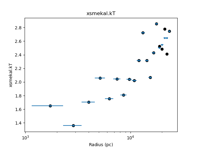
The results can be compared to the original, such as in the following plot, which shows that the temperature profile hasn’t changed significantly in the core, but some of the oscillations at large radii have been reduced (the black circles show the temperature values from the original fit):

>>> dep.fit_plot('xsmekal.kt', units='pc')
>>> rmid = (onion['rlo_phys'] + onion['rhi_phys']) / 2
>>> plt.scatter(rmid.to(u.pc), onion['xsmekal.kT', c='k')

Note

As the X-axis of the plot created by fit_plot() is in pc, the rmid value is expliclty converted to these units before plotting.

The results parameter of fit_plot could have been set to the variable onion to display the results of the previous fit, but there is no easy way to change the color of the points.

More shells could be tied together to try and further reduce the oscillations, or errors calculated, with either conf() or covar().

The parameter ties can be removed with untie_par():

>>> dep.untie_par('xsmekal.kt', 18)
Untying xsmekal_18.kT
>>> dep.untie_par('xsmekal.abundanc', 18)
Untying xsmekal_18.Abundanc
>>> dep.get_shells()[0:4]
[{'annuli': [19], 'dataids': [19]},
 {'annuli': [18], 'dataids': [18]},
 {'annuli': [17], 'dataids': [17]},
 {'annuli': [16], 'dataids': [16]}]