Installation
As of version 0.2.0, the deproject package
can be installed directly from PyPI. This requires CIAO 4.11 or later (in general the latest
release of CIAO should be used). The module can be used with the
standalone release of Sherpa, but it is only
useful if Sherpa has been built with XSPEC support which
is trickier to achieve than we would like.
Requirements
The package uses Astropy and SciPy, for units support and cosmological-distance calculations. It is assumed that Matplotlib is available for plotting.
It is strongly advised to use the latest CIAO (at the time of writing this is CIAO 4.14) installed with conda. Support for CIAO installed via the ciao-install script is limited.
Using pip
It should be as simple as starting the CIAO environment - this depends on whether CIAO was installed via ciao-install or conda - and then saying:
pip install deproject
This approach should also work if you are using the standalone version of Sherpa.
Manual installation
The source is available on github at https://github.com/sherpa-deproject/deproject, with releases available at https://github.com/sherpa-deproject/deproject/releases.
After downloading the source code (whether from a release or by cloning the repository) and moving into the directory (deproject-<version> or deproject), installation just requires:
pip install .
Note
This command should only be run after setting up CIAO or whatever Python environment contains your Standalone Sherpa installation.
Test
The source installation includes a basic test suite, which can be run with
pytest
Example data
The example data can be download from either http://cxc.cfa.harvard.edu/contrib/deproject/downloads/m87.tar.gz or from GitHub. The source distribution includes scripts - in the examples directory - that can be used to replicate both the basic M87 example and the follow-on example combining annuli.
As an example (from within an IPython session, such as the Sherpa shell in CIAO):
>>> %run fit_m87.py
...
... a lot of screen output will whizz by
...
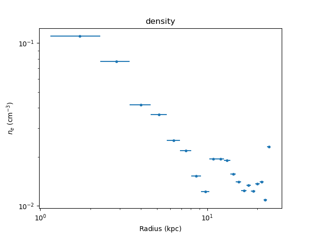
The current density estimates can then be displayed with:
>>> dep.density_plot()
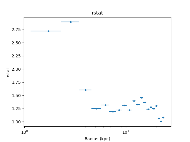
the reduced-statistic for the fit to each shell with:
>>> dep.fit_plot('rstat')
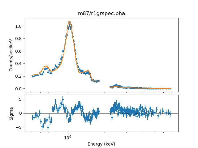
and the fit results for the first annulus can be displayed using the Sherpa functions:
>>> set_xlog()
>>> plot_fit_delchi(0)